Introduction to Word Embeddings: Problems and Theory

Making sense of Word Embeddings, how they solve problems and help machines understand language

LearnDataSci is reader-supported. When you purchase through links on our site, earned commissions help support our team of writers, researchers, and designers at no extra cost to you.

In the previous post, we introduced what word embeddings are and what they can do. This time, we'll try to make sense of them. What problem do they solve? How can they help computers understand natural language?

Understanding

See if you can guess what the word wapper means from how it's used in the following two sentences:

After running the marathon, I could barely keep my legs from wappering.
Thou'll not see Stratfort to-night, sir, thy horse is wappered out. (Or perhaps a more modern take: I can't drive you to Stratford tonight for I'm wappered out).

The second example is from the Oxford English Dictionary entry. If you haven't guessed, the word was probably more popular in the late-19th century. But it means to shake, especially from fatigue (and it might share the same linguistic roots as to waver). By now, you likely have a pretty good understanding of what to wapper means, if you like, even creating new sentences. Impressively, you probably didn't need me to explicitly tell you the definition; indeed, how many words in this sentence did you learn by reading a dictionary entry? We learn what words mean from their surrounding contexts. This implies that even though it appears that the meaning of a word is intrinsic to the word, some of the meaning of a word also exists in its context. Words, like notes on an instrument, do have their individual tones. But it is their relationship with each other---their interplay---that gives way to fuller music. Context enriches meaning. So, take a context, \[\textrm{After running the marathon, I could barely keep my legs from ____________.}\] We should have a sense of what words could fill the blank. Much more likely to appear are words like shaking, trembling, and of course, wappering. Especially compared to nonsense like pickled, big data, or even pickled big data. In short, the higher probability of appearing in this context corresponds to greater shared meaning. From this, we can deduce the distributional hypothesis: words that share many contexts tend to have similar meaning. What does this mean for a computer trying to understand words? Well, if it can estimate how likely a word is to appear in different contexts, then for most intents and purposes, the computer has learned the meaning of the word.¹ Mathematically, we want to approximate the probability distribution of \[p(\textrm{ word } | \textrm{ context }) \quad\textrm{ or }\quad p(\textrm{ context }|\textrm{ word }).\] Then, the next time the computer sees a specific context $c$, it can just figure out which words have the highest probability of appearing, $p(\textrm{ word }|\ c\ )$.

Challenges

The straightforward and naive approach to approximating the probability distribution is:

step 1: obtain a huge training corpus of texts,
step 2: calculate the probability of each (word,context) pair within the corpus.

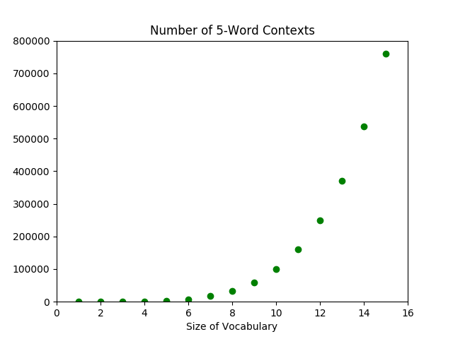
The underlying (bad) assumption? The probability distribution learned from the training corpus will approximate the theoretical distribution over all word-context pairs. However, if we think about it, the number of contexts is so great that the computer will never see a vast majority of them. That is, many of the probabilities $p(\textrm{ word } |\ c\ )$ will be computed to be 0. This is mostly a terrible approximation. The problem we've run into is the curse of dimensionality. The number of possible contexts grows exponentially relative to the size of our vocabulary---when we add a new word to our vocabulary, we more or less multiply the number of contexts we can make.²

**Figure 1.** The exponential growth of the number of contexts with respect to the number of words.

We overcome the curse of dimensionality with word embeddings, otherwise known as distributed representations of words. Instead of focusing on words as individual entities to be trained one-by-one, we focus on the attributes or features that words share. For example, king is a noun, singular and masculine. Of course, many words are masculine singular nouns. But as we add more features, we narrow down on the number of words satisfying each of those qualities. Eventually, if we consider enough features, the collection of features a word satisfies will be distinct from that of any other word.³ This lets us uniquely represent words by their features. As a result, we can now train features instead of individual words.⁴ This new type of algorithm would learn more along the lines of in this context, nouns having such and such qualities are more likely to appear instead of we're more likely to see words X, Y, Z. And since many words are nouns, each context teaches the algorithm a little bit about many words at once. In summary, every word we train actually recalls a whole network of other words. This allows us to overcome the exponential explosion of word-context pairs by training an exponential number of them at a time.⁵

A New Problem

In theory, representing words by their features can help solve our dimensionality problem. But, how do we implement it? Somehow, we need to be able to turn every word into a unique feature vector, like so:

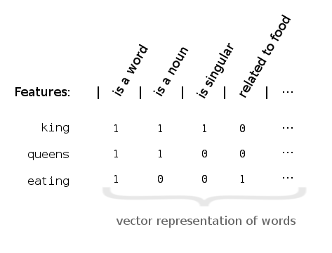
**Figure 1.** The feature vector of the word *king* would be $\langle 1, 1, 1,0,\dotsc\rangle$.

But features like is a word isn't very helpful; it doesn't contribute to forming a unique representation. One way to ensure uniqueness is by looking at a whole lot of specific features. Take is the word 'king' or is the word 'gastroenteritis', for example. That way, every word definitely corresponds to a different feature vector:

**Figure 2.** An inefficent representation defeating the purpose of word embeddings.

This isn't a great representation though. Not only is this a very inefficient way to represent words, but it also fails to solve the original dimensionality problem. Although every word still technically recalls a whole network of words, each network contains only one word! Constructing the right collection of features is a hard problem. They have to be not too general, not too specific. The resulting representation of each word using those features should be unique. And, we should limit the number of features to between 100-1000, usually. Furthermore, even though it's simpler to think about binary features that take on True/False values, we'll actually want to allow a spectrum of feature values. In particular, any real value. So, feature vectors are also actually vectors in a real vector space.

A New Solution

The solution to feature construction is: don't. At least not directly.⁶ Instead, let's revisit the probability distributions from before: \[p(\textrm{ word }|\textrm{ context }) \quad\textrm{and}\quad p(\textrm{ context }|\textrm{ word }).\] This time, words and contexts are represented by feature vectors: \[\textrm{word}_i = \langle \theta_{i,1}, \theta_{i,2}, \dotsc, \theta_{i,300}\rangle,\] which are just a collection of numbers. This turns the probability distributions from a functions over categorical objects (i.e. individual words) into a function over numerical variables $\theta_{ij}$. This is something that allows us to bring in a lot of existing analytical tools---in particular, neural networks and other optimization methods. The short version of the solution: from the above probability distributions, we can calculate the probability of seeing our training corpus, $p(\textrm{corpus})$, which had better be relatively large. We just need to find the values for each of the $\theta_{ij}$'s that maximize $p(\textrm{corpus})$. These values for $\theta_{ij}$ give precisely the feature representations for each word, which in turn lets us calculate $p( \textrm{ word }|\textrm{ context })$. Recall that this in theory teaches a computer the meaning of a word!

A Bit of Math

In this section, I'll give enough details for the interested reader to go on and understand the literature with a bit more ease. Recall from previously, we have a collection of probability distributions that are functions over some $\theta_{ij}$'s. The literature refers to these $\theta_{ij}$'s as parameters of the probability distributions $p(w|c)$ and $p(c|w)$. The collection of parameters $\theta_{ij}$'s is often denoted by a singular $\theta$, and the parametrized distributions by $p(w|c;\theta)$ and $p(c|w;\theta)$.⁷ If the goal is to maximize the probability of the training corpus, let's first write $p(\textrm{corpus};\theta)$ in terms of $p(c|w;\theta)$. There are a few different approaches. But in the simplest, we think of a training corpus as an ordered list of words, $w_1, w_2, \dotsc, w_T$. Each word in the corpus $w_t$ has an associated context $C_t$, which is a collection of surrounding words.

\[\begin{align*} \textrm{corpus: }\quad w_1\ | \ w_2\ | \ w_3\ | \quad \dotsm \quad & w _t \quad \dotsm \quad |\ w_{T-2} \ | \ w_{T-1} \ | \ w_T\\ & \,\Big\downarrow\\ \textrm{context of $w_t$: }\quad \big[ w_{t-n}\ \dotsm\ w_{t-1}\big]\ &w_t \ \big[w_{t+1}\ \dotsm\ w_{t+n} \big] \end{align*}\]

Diagram 1. A corpus is just an ordered list of words. The context $C_t$ of $w_t$ is a collection of words around it.⁸

For a given word $w_t$ in the corpus, the probability of seeing another word $w_c$ in its context is $p(w_c|w_t;\theta)$. Therefore, the probability that a word sees all of the surrounding context words $w_c$ in the training corpus is \[\prod_{w_c \in C_t} p(w_c|w_t;\theta).\] To get the total probability of seeing our training corpus, we just take the product over all words in the training corpus. Thus, \[p(\textrm{corpus};\theta) = \prod_{w_t}\prod_{w_c \in C_t} p(w_c|w_t;\theta).\] Now that we have the objective function, $f(\theta) = p(\textrm{corpus};\theta)$, it's just a matter of choosing the parameters $\theta$ that maximize $f$.⁹ Depending on how the probability distribution is parametrized by $\theta$, this optimization problem can be solved using neural networks. For this reason, this method is also called a neural language model (NLM). There are actually more layers of abstraction and bits of brilliance between theory and implementation. While I hope that I've managed to give you some understanding on where research is proceeding, the successes of the current word embedding methods are still rather mysterious. The intuition we've developed on the way is still, as Goldberg, et. al. wrote, "very hand-wavy" (Goldberg 2014). Still, perhaps this can help you have some intuition for what's going on behind all the math when reading the literature. A lot more has been written on this subject too; you can also take a look below where I list more resources I found useful.

Resources & References

I focused mainly on word2vec while researching neural language models. However, do keep in mind that word2vec was just one of the earlier and possibly more famous models. To understand the theory, I quite liked all of the following. Approximately in order of increasing specificity,

Radim Řehůřek's introductory post on word2vec. He also wrote and optimized the word2vec algorithm for Python, which he notes sometimes exceeds the performance of the original C code.
Chris McCormick's word2vec tutorial series, which goes into much more depths on the actual word2vec algorithm. He writes very clearly, and he also provides a list of resources.
Goldberg and Levy 2014, word2vec Explained, which helped me formulate my explanations above.
Sebastian Ruder's word embedding series. I found this series comprehensive but really accessible.
Bojanowski 2016, Enriching word vectors with subword information. This paper actually is for Facebook's fastText (which Mikolov is a part of), but it is based in part on word2vec. I found the explanation of word2vec's model in Section 3.1 transparent and concise.
Levy 2015, Improving distributional similarity with lessons learned from word embeddings points out that actually, the increased performance of word2vec over previous word embeddings models might be a result of "hyperparameter optimizations," and not necessarily in the algorithm itself.

[expand title="Expand here to see the he references I cited above" trigclass="arrowright"] [Bengio 2003] Bengio, Yoshua, et al. "A neural probabilistic language model." Journal of machine learning research 3.Feb (2003): 1137-1155. [Bojanowski 2016] Bojanowski, Piotr, et al. "Enriching word vectors with subword information." arXiv preprint arXiv:1607.04606 (2016). [Goldberg 2014] Goldberg, Yoav, and Omer Levy. "word2vec Explained: deriving Mikolov et al.'s negative-sampling word-embedding method." arXiv preprint arXiv:1402.3722 (2014). [Goodfellow 2016] Goodfellow, Ian, Yoshua Bengio, and Aaron Courville. Deep learning. MIT press, 2016. [Hamilton 2016] Hamilton, William L., et al. "Inducing domain-specific sentiment lexicons from unlabeled corpora." arXiv preprint arXiv:1606.02820 (2016). [Kusner 2015] Kusner, Matt, et al. "From word embeddings to document distances." International Conference on Machine Learning. 2015. [Levy 2015] Levy, Omer, Yoav Goldberg, and Ido Dagan. "Improving distributional similarity with lessons learned from word embeddings." Transactions of the Association for Computational Linguistics 3 (2015): 211-225. [Mikolov 2013a] Mikolov, Tomas, Wen-tau Yih, and Geoffrey Zweig. "Linguistic regularities in continuous space word representations." hlt-Naacl. Vol. 13. 2013. [Mikolov 2013b] Mikolov, Tomas, et al. "Efficient estimation of word representations in vector space." arXiv preprint arXiv:1301.3781 (2013). [Mikolov 2013c] Mikolov, Tomas, et al. "Distributed representations of words and phrases and their compositionality." Advances in neural information processing systems. 2013. [Mikolov 2013d] Mikolov, Tomas, Quoc V. Le, and Ilya Sutskever. "Exploiting similarities among languages for machine translation." arXiv preprint arXiv:1309.4168 (2013). [Mnih 2012] Mnih, Andriy, and Yee Whye Teh. "A fast and simple algorithm for training neural probabilistic language models." arXiv preprint arXiv:1206.6426 (2012). [Rong 2014] Rong, Xin. "word2vec parameter learning explained." arXiv preprint arXiv:1411.2738 (2014). [/expand]

Footnotes

And let's not get into any philosophical considerations of whether the computer really understands the word. Come to think of it, how do I even know you understand a word of what I'm saying? Maybe it's just a matter of serendipity that the string of words I write make sense to you. But here I am really talking about how to oil paint clouds, and you think that I'm talking about machine learning.↩
Consider a 20-word context. If we assume that the average English speaker's vocabulary is 25,000 words, then the increase of 1 word corresponds to an increase of about $7.2\times 10^{84}$ contexts, which is actually more than the number of atoms in the universe. Of course, most of those contexts wouldn't make any sense.↩
The algorithm used by the Google researchers mentioned above assumes 300 features.↩
The term distributed representation of words comes from this: we can now represent words by their features, which are shared (i.e. distributed) across all words. We can imagine the representation as a feature vector. For example, it might have a 'noun bit' that would be set to 1 for nouns and 0 for everything else. This is, however, a bit simplified. Features can take on a spectrum of values, in particular, any real value. So, feature vectors are actually vectors in a real vector space.↩
The distributed representations of words "allows each training sentence to inform the model about an exponential number of semantically neighboring sentences," (Bengio 2003).↩
This also means that there's probably not a 'noun bit' in our representation, like in the figures above. There might not be any obvious meaning to each feature.↩
The softmax function is often chosen as the ideal probability distribution. Let $w_t$ be the vector representation of a word, and let $C_t$ be the collection of words that have appeared in the context of $w_t$. Then, \[p(w_c|w_t;\theta) = \frac{e^{w_c \cdot w_t}}{\sum_{w_{c'} \in C_t} e^{w_{c'} \cdot w_t}}.\] But other related functions are used in practice (for computational reason). The point here is that the parameters $\theta$ are then optimized with respect to the selected distribution function.↩
One can control the algorithm by specifying different hyperparameters: do we care about order of words? How many surrounding words do we consider? And on.↩
This maximization problem is often equivalently written as \[\operatorname*{arg\,max}_\theta \sum_{w_t} \sum_{C_t} \log p(w_c|w_t;\theta).\]↩

Start Learning for Free

Meet the Authors

Aaron So C.S. Graduate Student at Columbia University

Back to blog index

Introduction to Word Embeddings: Problems and Theory