

Data Scientist
From Good to Great Data Science, Part 1: Correlations and Confidence
With the aid of some hospital data, part one describes how just a little inexperience in statistics could result in two common mistakes
import pandas as pd
from scipy import stats
import mathIntroduction
As a data scientist you'll spend a lot of time answering questions with data. I currently work as a data scientist in the healthcare industry, providing metrics and building models for hospitals and healthcare related organizations. In my practice most of my time is spent doing two things:
- Translating qualitative business questions into rigorous solutions that can be generated with data
- Implementing these solutions programmatically
I'm going to walk you through two questions that I've actually been asked on the job:
- Should my hospital focus more on improving its mortality rate?
- Which pharmacists are handing out too many opioids?
What they both have in common is that there's a right way and a wrong way to do them. Further, it's very easy to answer these questions the wrong way and have your mistakes go unnoticed. As you'll see, the difference between great and average answers to these questions is a having a little bit of a mathematical background.
Jupyter notebook and data for this article on GitHub
Problem Statement 1:
The Centers for Medicare & Medicaid Services (CMS) is responsible for rating hospitals based off of quality and performance metrics.
They provide various metrics to estimate hospital performance and one overarching metric known as the quality_rating. Another less important rating is the mortality_rate.
Suppose you're tasked with investigating the relationship between a hospital's quality_rating and its mortality_rate to answer the first question I mentioned above. How much does a hospital's mortality rate affect its overall quality_rating? Assume the following about your data:
quality_rating: A numerical value in the range (1, 2, 3, 4, 5)mortality_rate: One of the following values:- above_average
- average
- below_average
And assume you're given the data below:
ratings_df = pd.read_csv('hospital_ratings.csv').drop(columns='Unnamed: 0')
print('Number of Hospitals: {}'.format(len(ratings_df.index)))
ratings_df.head(10)Number of Hospitals: 100| mortality_rate | quality_rating | |
|---|---|---|
| 0 | average | 1 |
| 1 | below_average | 4 |
| 2 | above_average | 1 |
| 3 | average | 4 |
| 4 | average | 4 |
| 5 | below_average | 5 |
| 6 | below_average | 4 |
| 7 | below_average | 4 |
| 8 | average | 3 |
| 9 | average | 5 |
As you can see, each row represents a hospital. Each hospital has a mortality rate and quality score. The premise is to compare mortality_rate and quality_rating so a key statistical tool should be jumping to your head. Correlation.
This is the first step of reducing our qualitative question into quantitative terms. I urge you to take a stab at the problem at this point — or at least flesh out a complete plan to answering the question:
What's the correlation between these two metrics?
Did you arrive at a solution? Lets walk through this together.
Encoding mortality rate
There are arguably two steps remaining in this problem. First, we should note that our mortality_rate column contains ordinal data. We can only perform correlation on numerical data so we'll have to do something about this.
Let's encode our data in some way that preserves its ordinal relationship. In other words, we want to our encoding for below average mortality_rate to be numerically superior to our encoding for above average mortality_rate (Note that a hospital having a lower mortality rate is better).
How did you tackle encoding your data? There's an infinite amount of options:
For instance:
'below average' --> 5
'average' --> 3
'above average' --> 1or:
'below average' --> 3
'average' --> 2
'above average' --> 1or maybe:
'below average' --> 1
'average' --> 0
'above average' --> -1If you made the decision to encode your data, what option did you settle on? Which one is correct? The correct answer is none of them — or all of them I guess...
I'll explain why in a bit. But for now, let’s just continue with mapping to last option: mapping to the set: (-1, 0, 1).
MORTALITY_MAP = {
'below_average': 1,
'average': 0,
'above_average': -1
}
ratings_df['mortality_rate'] = ratings_df['mortality_rate'].map(MORTALITY_MAP) # apply the map
ratings_df.head()| mortality_rate | quality_rating | |
|---|---|---|
| 0 | 0 | 1 |
| 1 | 1 | 4 |
| 2 | -1 | 1 |
| 3 | 0 | 4 |
| 4 | 0 | 4 |
The last step to this problem is (deceptively) the simplest. Now we just need to correlate our two columns right?
ratings_df.corr()| mortality_rate | quality_rating | |
|---|---|---|
| mortality_rate | 1.000000 | 0.473712 |
| quality_rating | 0.473712 | 1.000000 |
Not quite. We've made a huge assumption about our data. We've assumed that our data was anything more than ordinal.
Non-parametric correlation
As a data scientist, you should be familiar with the concept of parametric and non-parametric statistics. Most statistical correlations will default to a parametric correlation method known as pearson. In our case, we need to use a non-parametric correlation known as spearman.
This non-parametric method assumes that our data is nothing more than ordinal. In other words, no matter what mapping we make, the spearman correlation will return the same result — so long as the order is preserved after mapping.
If we specify that we need to use the spearman correlation method, then we notice a drastic change in results:
ratings_df.corr(method='spearman')| mortality_rate | quality_rating | |
|---|---|---|
| mortality_rate | 1.000000 | 0.379098 |
| quality_rating | 0.379098 | 1.000000 |
We've just dropped the correlation by about 10%. That's a drastic difference!
Had you reported this correlation using pearson as opposed to spearman, you might have seriously mislead a customer or coworker.
This goes to show that having a strong statistical background is essential for the data science role. Such a deceptively simple problem had a key mathematical step that's often overlooked.
Problem Statement 2:
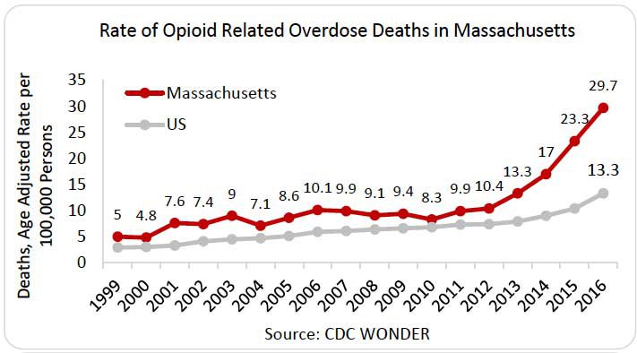
You have millions of pharmaceutical records for the past 5 years in Massachusetts, a state well known for its opioid abuse problem. For this reason, it would be very useful if you could identify pharmacists who are prescribing too many opioids.
You're tasked with the following:
Generate a list of pharmacists who are overprescribing opioids.
Seems simple enough. Suppose you have the following dataset:
prescribers_df = pd.read_csv('prescriptions.csv').drop(columns='Unnamed: 0')
prescribers_df.head(10)| prescriber_id | num_opioid_prescriptions | num_prescriptions | |
|---|---|---|---|
| 0 | BDRSDDB2&RA | 4 | 7 |
| 1 | 3$N3WG4&BBO | 25 | 28 |
| 2 | S2NGGOGBRB4 | 1 | 1 |
| 3 | S2NGGOGBRB4 | 18 | 22 |
| 4 | NBORABOESOI | 1 | 1 |
| 5 | 4O4EAGWROGB | 20 | 30 |
| 6 | WPOARS4GW9I | 11 | 12 |
| 7 | PDS$GG9GOGA | 29 | 37 |
| 8 | BBP34DOGADB | 1 | 1 |
| 9 | S$BO&OGO99O | 16 | 19 |
Each row represents a days worth of prescriptions
And we have the following columns:
prescriber_id: A random code that identifies pharmacistsnum_opioid_prescriptions: The number of opioid prescriptions prescribed on a given daynum_prescriptions: The number of total prescriptions prescribed on a given day
Grouping prescribers
The first thing we should note is that prescriber_id does not contain unique values as prescribers may have prescribed drugs over multiple days. Since this metric is on a prescriber level — not a daily level — we should fix that with a pandas groupby.
prescribers_df = prescribers_df.groupby('prescriber_id').agg('sum')
prescribers_df.head(10)| num_opioid_prescriptions | num_prescriptions | |
|---|---|---|
| prescriber_id | ||
| $39AGIIOGO2 | 15 | 22 |
| $DG2GOGDD9D | 14 | 18 |
| $OBDNSADD96 | 37 | 57 |
| &OB | 16 | 20 |
| &64O2OASRNA | 22 | 23 |
| &AGO$DEOPRR | 47 | 58 |
| &OS2DN4DADO | 1 | 1 |
| &SOEB4RODOG | 39 | 51 |
| 2BDPWROOBOR | 13 | 17 |
| 3$N3WG4&BBO | 32 | 39 |
Much better. Now the task at hand is to rank prescribers on the basis of how many opioids they prescribe. But prescribers prescribe different amounts of drugs. This hints that we should now take each prescriber's opioid prescription ratio. Let's do just that.
Opioid prescription ratio
prescribers_df['opioid_prescription_ratio'] = (prescribers_df['num_opioid_prescriptions'] /
prescribers_df['num_prescriptions'])Pandas made that extremely easy. So we're done right? Just sort the prescribers by opioid_ratio and tie this task off?
prescribers_df.sort_values('opioid_prescription_ratio', ascending=False).head(10)| num_opioid_prescriptions | num_prescriptions | opioid_prescription_ratio | |
|---|---|---|---|
| prescriber_id | |||
| DE6WBN9W | 1 | 1 | 1.0 |
| 3NG4ONN46GO | 2 | 2 | 1.0 |
| 6W349S&GD&N | 1 | 1 | 1.0 |
| 4WA6NBOO&DB | 1 | 1 | 1.0 |
| NBORABOESOI | 1 | 1 | 1.0 |
| 4R9RDN2G6D9 | 1 | 1 | 1.0 |
| OAIGB9OGSE$ | 1 | 1 | 1.0 |
| PGWSD49S6OW | 1 | 1 | 1.0 |
| BO&2BGDNGO& | 1 | 1 | 1.0 |
| 4BBA2OGP9G6 | 1 | 1 | 1.0 |
Not quite. This data should raise some red flags for you.
Does it really make sense to rank a pharmacist as an abuser for prescribing 1 opioid out of 1 of their total prescriptions? Try to put into words exactly what's wrong with this situation. Why do we not want to report these prescribers as the worst offenders? Hopefully the answer you arrive at is something along the lines of:
Because we don't have enough information to judge them.
Imagine you were sitting in a pharmacy watching a pharmacist (let's call them "Bill") perform their job. Suppose you want to report Bill if he prescribes too many opioids.
A customer walks in and Bill prescribes them hydrocodone (a common opioid). It'd be silly to report Bill immediately for this. You'd want to wait and see more of Bill's actions before you judged him because you're not confident in your findings yet.
Confidence is a key word here as we'll soon find out.
Building confidence
So how do we fix this issue?
Statistically speaking, prescribing an opioid or not can be though of as a Bernouli parameter (a fancy term for something that's binary in value — either true or false). And given the number of observations of a bernoulli parameter, we want to predict this parameter's true value.
By "true value" I mean the actual value that prescriber's opioid_prescription_ratio would converge to if we had enough observations. The "true value" in our example with Bill would be equivalent to Bill's opioid_prescription_ratio if we were able to watch and record his actions for a very long time — like a year.
If you've taken a statistics or good data science course you're probably familiar with the concept of confidence intervals. If not, in simplest terms, a confidence interval is just a measure of mathematical confidence attached to a range that you believe an unknown value exists within.
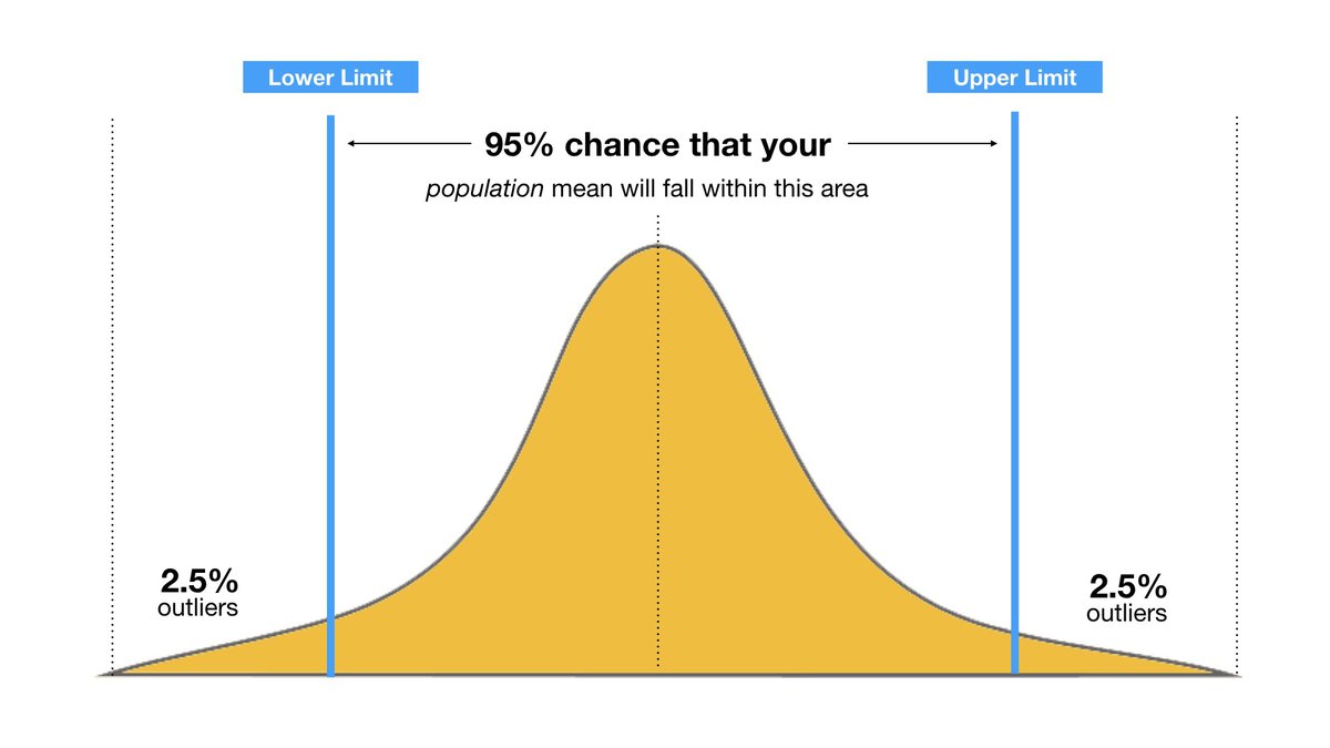
For example, I could be 95% confident that tomorrow's temperature will fall between 40 Fahrenheit and 70 Fahrenheit.
In 1927 mathematician Edwin Wilson applied the concept of confidence intervals to Bernoulli parameters. This means we can guess the true value of a pharmacists opioid_prescription_ratio given the amount of data we have on them!
Here's the formula:
Wilson Confidence Interval Lower Bound:
- $\hat{p}$ – pronounced p-hat – is the percentage of positive observations (opioid prescriptions in our case).
- $z$ is the confidence level of our choosing (.95 or higher is standard)
- and $n$ is the total number of observations (total number of prescriptions in our case).
The formula looks intimidating but it's intuitive if you take the time to walk through it. Explaining the mathematics behind why this formula works is worth an entire discussion itself and is thus out of scope. So we'll just focus on applying it below.
def wilson_ci_lower_bound(num_pos, n, confidence=.95):
if n == 0:
return 0
z = stats.norm.ppf(1 - (1 - confidence) / 2) # Establish a z-score corresponding to a confidence level
p_hat = num_pos / n
# Rewrite formula in python
numerator = p_hat + (z**2 / (2*n)) - (z * math.sqrt((p_hat * (1 - p_hat) + (z**2 / (4*n))) / n))
denominator = 1 + ((z**2) / n)
return numerator / denominatorLet's apply this formula to our dataframe with 95% confidence, creating a new column
prescribers_df['wilson_opioid_prescription_ratio'] = prescribers_df \
.apply(lambda row: wilson_ci_lower_bound(row['num_opioid_prescriptions'], row['num_prescriptions']), axis=1)
prescribers_df.sort_values('wilson_opioid_prescription_ratio', ascending=False).head(10)| num_opioid_prescriptions | num_prescriptions | opioid_prescription_ratio | wilson_opioid_prescription_ratio | |
|---|---|---|---|---|
| prescriber_id | ||||
| 4BOSRODA$GI | 49 | 52 | 0.942308 | 0.843575 |
| EDB3BB2AGAA | 41 | 44 | 0.931818 | 0.817750 |
| SGSGRIIBDBA | 31 | 33 | 0.939394 | 0.803938 |
| &64O2OASRNA | 22 | 23 | 0.956522 | 0.790088 |
| SBO3WOOBIBP | 22 | 23 | 0.956522 | 0.790088 |
| GSP3D&P$DNP | 21 | 22 | 0.954545 | 0.782020 |
| GOADO3OE | 33 | 36 | 0.916667 | 0.781733 |
| RADBOGNS4DS | 24 | 26 | 0.923077 | 0.758584 |
| RNA6SBBAG6B | 18 | 19 | 0.947368 | 0.753613 |
| IEBIBWSD2$B | 18 | 19 | 0.947368 | 0.753613 |
Amazing! Now these are the results we would want to report.
While there are plenty of prescribers with 1/1 or 2/2 opioid prescriptions, they now appear at the bottom of our rankings – which is intuitive. While our highest ranking prescribers have a lower opioid_prescription_ratio than some other prescribers, the rankings now take into account a notion of mathematical confidence.
Both approaches to this problem — with or without using confidence intervals — are technically acceptable. However, it's easy to see that approaching the problem with a mathematical background yielded much more valuable results.
In Conclusion...
A large part of the data science job is translating open and interpretable questions into quantitative, rigorous terms.
As both of these examples have demonstrated, sometimes it’s not such an easy task and many data scientists often fall short in this regard. It’s very easy to fall into the trap of using parametric correlation in a non-parametric scenario. And it’s very easy to naively sort a list of Bernoulli trials without taking into account the number of observations for each trial. In fact, it happens more often than you’d think in practice.
Part of what separates a good data scientist from a great data scientist is having the mathematical background and intuition to identify and act upon situations like this. Often times what can make the difference between a solution and a great solution in data science is leveraging the right mathematical tools in the right context.
Meet the Authors

Studied mathematics at Northeastern University, with a research focus in combinatorics and linear algebra. Currently working as a data scientist for a start-up in the greater Boston area with a passion for mathematics, data science, formal verification, and algorithm design.