
Data Scientist
Intro to Feature Engineering for Machine Learning with Python
Feature Engineering is the process of transforming data to increase the predictive performance of machine learning models.
LearnDataSci is reader-supported. When you purchase through links on our site, earned commissions help support our team of writers, researchers, and designers at no extra cost to you.
Introduction
You will learn:
By the end of this article you should know:
- Two primary methods for feature engineering
- How to use Pandas and Numpy to perform several feature engineering tasks in Python
- How to increase predictive performance of a real dataset using these tasks
Feature engineering is arguably the most important, yet overlooked, skill in predictive modeling. We employ it in our everyday lives without thinking about it!
Let me explain - let's say you're a bartender and a person comes up to you and asks for a vodka tonic. You proceed to ask for ID and you see the person's birthday is "09/12/1998". This information is not inherently meaningful, but you add up the number of years by doing some quick mental math and find out the person is 22 years old (which is above the legal drinking age). What happened there? You took a piece of information ("09/12/1998") and transformed it to become another variable (age) to solve the question you had ("Is this person allowed to drink?").
Feature engineering is exactly this but for machine learning models. We give our model(s) the best possible representation of our data - by transforming and manipulating it - to better predict our outcome of interest. If this isn’t 100% clear now, it will be a lot clearer as we walk through real examples in this article.
Definition
Feature Engineering is the process of transforming data to increase the predictive performance of machine learning models.
Importance
Feature engineering is both useful and necessary for the following reasons:
- Often better predictive accuracy: Feature engineering techniques such as standardization and normalization often lead to better weighting of variables which improves accuracy and sometimes leads to faster convergence.
- Better interpretability of relationships in the data: When we engineer new features and understand how they relate with our outcome of interest, that opens up our understanding of the data. If we skip the feature engineering step and use complex models (that to a large degree automate feature engineering), we may still achieve a high evaluation score, at the cost of better understanding our data and its relationship with the target variable.
Feature engineering is necessary because most models cannot accept certain data representations. Models like linear regression, for example, cannot handle missing values on their own - they need to be imputed (filled in). We will see examples of this in the next section.
Workflow
Every data science pipeline begins with Exploratory Data Analysis (EDA), or the initial analysis of our data. EDA is a crucial pre-cursor step as we get a better sense of what features we need to create/modify. The next step is usually data cleaning/standardization depending on how unstructured or messy the data is.
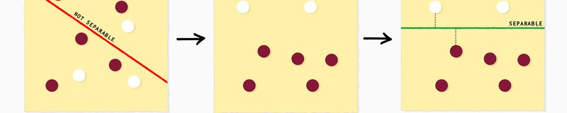
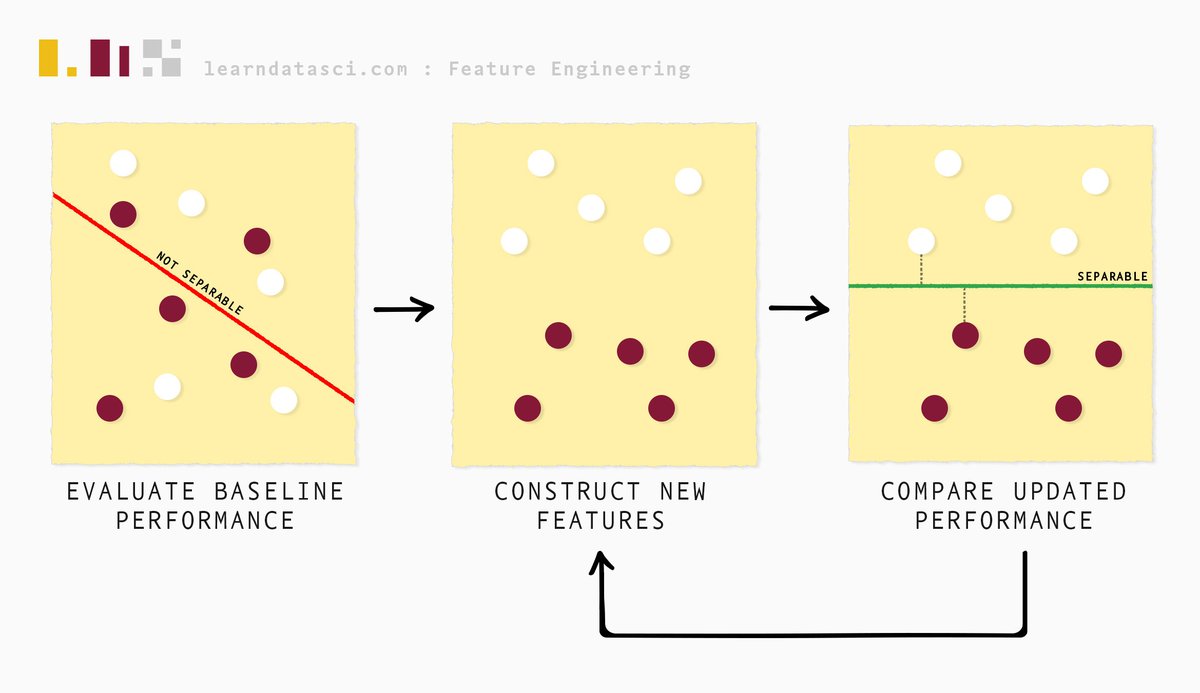
Feature engineering follows next and we begin that process by evaluating the baseline performance of the data at hand. We then iteratively construct features and continuously evaluate model performance (and compare it with the baseline performance) through a process called feature selection, until we are satisfied with the results.
What this article does and does not cover
Feature engineering is a vast field as there are many domain-specific tangents. This article covers some of the popular techniques employed in handling tabular datasets. We do not cover feature engineering for Natural Language Processing (NLP), image classification, time-series data, etc.
The two approaches to feature engineering
There are two main approaches to feature engineering for most tabular datasets:
- The checklist approach: using tried and tested methods to construct features.
- The domain-based approach: incorporating domain knowledge of the dataset’s subject matter into constructing new features.
We will now look at these approaches in detail using real datasets. Note, these examples are quite procedural and focus on showing how you can implement it in Python. The case study following this section will show you a real end-to-end scenario use case of the practices we touch upon in this section.
Before we load the dataset, we import the following dependencies shown below.
# dependencies
import pandas as pd
import numpy as np
import matplotlib.pyplot as plt
import seaborn as sns
sns.set_theme()
sns.set_palette(sns.color_palette(['#851836', '#edbd17']))
sns.set_style("darkgrid")
from sklearn.preprocessing import MinMaxScaler
from sklearn.decomposition import PCA
from sklearn.linear_model import LinearRegression
from sklearn.metrics import mean_squared_error
from sklearn.model_selection import train_test_splitWe will now demonstrate the checklist approach using a dataset on supermarket sales. The original dataset, and more information about it, is linked here. Note, the dataset has been slightly modified for this tutorial.
df = pd.read_csv('data/supermarket_sales.csv')
df.head()| Invoice ID | Branch | City | Customer type | Gender | Product line | Unit price | Quantity | Tax 5% | Total | Date | Time | Payment | cogs | gross margin percentage | gross income | Rating | |
|---|---|---|---|---|---|---|---|---|---|---|---|---|---|---|---|---|---|
| 0 | 750-67-8428 | A | Yangon | Member | Female | Health and beauty | 74.69 | 7.0 | 26.1415 | 548.9715 | 1/5/19 | 13:08 | Ewallet | 522.83 | 4.761905 | 26.1415 | 9.1 |
| 1 | 226-31-3081 | C | Naypyitaw | Normal | Female | Electronic accessories | 15.28 | 5.0 | 3.8200 | 80.2200 | 3/8/19 | 10:29 | Cash | 76.40 | 4.761905 | 3.8200 | 9.6 |
| 2 | 631-41-3108 | A | Yangon | Normal | Male | Home and lifestyle | 46.33 | 7.0 | 16.2155 | 340.5255 | 3/3/19 | 13:23 | Credit card | 324.31 | 4.761905 | 16.2155 | 7.4 |
| 3 | 123-19-1176 | A | Yangon | Member | Male | Health and beauty | 58.22 | 8.0 | 23.2880 | 489.0480 | 1/27/19 | 20:33 | Ewallet | 465.76 | 4.761905 | 23.2880 | 8.4 |
| 4 | 373-73-7910 | A | Yangon | Normal | Male | Sports and travel | 86.31 | 7.0 | 30.2085 | 634.3785 | 2/8/19 | 10:37 | Ewallet | 604.17 | 4.761905 | 30.2085 | 5.3 |
The Checklist Approach
Numeric Aggregations
Numeric aggregation is a common feature engineering approach for longitudinal or panel data - data where subjects are repeated. In our dataset, we have categorical variables with repeated observations (for example, we have multiple entries for each supermarket branch).
Numeric aggregation involves three parameters:
- Categorical column
- Numeric column(s) to be aggregated
- Aggregation type: Mean, median, mode, standard deviation, variance, count etc.
The below code chunk shows three examples of numeric aggregations based on mean, standard deviation and count respectively.
In the following block our three parameters are:
- Branch – categorical column, which we're grouping by
- Tax 5%, Unit Price, Product line, and Gender – numeric columns to be aggregated
- Mean, standard deviation, and count – aggregations to be used on the numeric columns
Below, we group by Branch and perform three statistical aggregations (mean, standard deviation, and count) by transforming the numeric columns of interest. For example, in the first column assignment, we calculate the mean Tax 5% and mean Unit price for every branch, which gives us two new columns - tax_branch_mean and unit_price_mean in the data frame.
# Numeric aggregations
grouped_df = df.groupby('Branch')
df[['tax_branch_mean','unit_price_mean']] = grouped_df[['Tax 5%', 'Unit price']].transform('mean')
df[['tax_branch_std','unit_price_std']] = grouped_df[['Tax 5%', 'Unit price']].transform('std')
df[['product_count','gender_count']] = grouped_df[['Product line', 'Gender']].transform('count')And we see the features we've just created below.
df[['Branch', 'tax_branch_mean', 'unit_price_mean', 'tax_branch_std',
'unit_price_std', 'product_count', 'gender_count']].head(10)| Branch | tax_branch_mean | unit_price_mean | tax_branch_std | unit_price_std | product_count | gender_count | |
|---|---|---|---|---|---|---|---|
| 0 | A | 14.894393 | 54.937935 | 11.043263 | 26.203576 | 331 | 342 |
| 1 | C | 16.052367 | 56.645583 | 12.531470 | 27.247291 | 308 | 328 |
| 2 | A | 14.894393 | 54.937935 | 11.043263 | 26.203576 | 331 | 342 |
| 3 | A | 14.894393 | 54.937935 | 11.043263 | 26.203576 | 331 | 342 |
| 4 | A | 14.894393 | 54.937935 | 11.043263 | 26.203576 | 331 | 342 |
| 5 | C | 16.052367 | 56.645583 | 12.531470 | 27.247291 | 308 | 328 |
| 6 | A | 14.894393 | 54.937935 | 11.043263 | 26.203576 | 331 | 342 |
| 7 | C | 16.052367 | 56.645583 | 12.531470 | 27.247291 | 308 | 328 |
| 8 | A | 14.894393 | 54.937935 | 11.043263 | 26.203576 | 331 | 342 |
| 9 | B | 15.277808 | 55.743474 | 11.557958 | 26.136309 | 321 | 333 |
Note: since we're viewing a column subset of the full df, it looks like there are duplicate rows. When the rest of the columns are visible you'll notice there aren't duplicate rows, but there are still duplicate values. This is by design.
Choosing numeric aggregation parameters
How do we pick which three parameters to use? Well, that will depend on your domain knowledge and your understanding of the dataset. For example, in this dataset, if you feel like the variation in the average (aggregation type) Rating (numeric variable) based on the Branch (categorical column) is important in predicting gross income (target variable), create the feature! If you feel like the count of the products in the Product Line, by branch, is important in informing gross income, encode that as a feature!
Now if you can test as many combinations of the three parameters - go ahead - as long as you are meticulous at selecting only those features that have enough predictive power i.e. be sure to have a rigorous feature selection process.
Below we can see a couple of the columns we created (tax_branch_mean and unit_price_mean). They are aggregations based on the Branch variable.
df[['Tax 5%', 'Unit price', 'Branch', 'tax_branch_mean', 'unit_price_mean']]| Tax 5% | Unit price | Branch | tax_branch_mean | unit_price_mean | |
|---|---|---|---|---|---|
| 0 | 26.1415 | 74.69 | A | 14.894393 | 54.937935 |
| 1 | 3.8200 | 15.28 | C | 16.052367 | 56.645583 |
| 2 | 16.2155 | 46.33 | A | 14.894393 | 54.937935 |
| 3 | 23.2880 | 58.22 | A | 14.894393 | 54.937935 |
| 4 | 30.2085 | 86.31 | A | 14.894393 | 54.937935 |
| ... | ... | ... | ... | ... | ... |
| 998 | 3.2910 | 65.82 | A | 14.894393 | 54.937935 |
| 999 | 30.9190 | 88.34 | A | 14.894393 | 54.937935 |
| 1000 | 30.9190 | 88.34 | A | 14.894393 | 54.937935 |
| 1001 | 5.8030 | NaN | A | 14.894393 | 54.937935 |
| 1002 | 30.4780 | 87.08 | B | 15.277808 | 55.743474 |
1003 rows × 5 columns
But why is all of this necessary?
Now before I go on any further, you may be wondering why this is even necessary - aren't good models designed to take all of these aggregations into account? To an extent, yes, but not always. It depends a lot on the size and dimensionality (number of columns) of your dataset. The larger the dataset, the more features (by several orders of magnitude) you can create. When there are too many features, the model has too many competing signals to predict the target variable.
Feature engineering tries to explicitly focus the model's attention on certain features. To summarize, feature engineering is not about creating "new" information, but rather directing and/or focusing the model's attention on certain information, that you as the data scientist judge to be important.
Indicator Variables and Interaction Terms
Following the same pattern of thinking as numeric aggregations, we can construct indicator variables and interaction terms.
Indicator variables only take on the value 0 or 1 to indicate the absence or presence of some information.
For example, below we define an indicator variable unit_price_50 to indicate if the product has a unit price greater than 50. To put it into perspective, think of an e-commerce store having free shipping on all orders above $50; this may be useful information in predicting customer behavior and worth an explicit definition for the model.
Interaction terms are created based on the presence of interaction effects between two or more variables. This is largely driven by domain expertise, although there are statistical tests to help determine them (which is beyond the scope of this article). For example, while free shipping may affect customer rating, free shipping combined with quantity may have a different effect on customer rating, which would be useful to encode (assuming customer rating is the target variable in this case). Below we define the variable unit_price_50 * qty to be exactly that.
We use np.where() to create an indicator variable unit_price_50 that encodes 1 when unit price is above 50 and 0 otherwise.
df['unit_price_50'] = np.where(df['Unit price'] > 50, 1, 0)
df['unit_price_50 * qty'] = df['unit_price_50'] * df['Quantity']df[['unit_price_50', 'unit_price_50 * qty']].head()| unit_price_50 | unit_price_50 * qty | |
|---|---|---|
| 0 | 1 | 7.0 |
| 1 | 0 | 0.0 |
| 2 | 1 | 7.0 |
| 3 | 1 | 8.0 |
| 4 | 1 | 7.0 |
Numeric Transformations
Some data scientists don't consider numeric transformations to fall under feature engineering. This is because many models, especially the newer ones like tree-based models (decision trees, random forests, etc.), are not impacted by these transformations. In other words, performing these transformations does nothing to improve predictive performance. But for other models such as linear regression, these transformations can make a big difference as they are sensitive to the scale of their variables.
Below we construct a new variable log_cogs to correct for the right skew in the variable cogs. The effect is shown in the plots below the code chunk.
We can also do other transformations such as squaring a variable (shown in the code chunk below) if we believe the relationship between a predictor and target variable is not linear, but quadratic in nature (as a predictor variable changes, target variable changes by an order of 2).
We can even have cubed variables or any n degree polynomial term - it is up to your discretion and domain knowledge.
# numeric transformations
df['log_cogs'] = np.log(df['cogs'] + 1)
df['gross income squared'] = np.square(df['gross income'])df[['cogs', 'log_cogs', 'gross income', 'gross income squared']].head()| cogs | log_cogs | gross income | gross income squared | |
|---|---|---|---|---|
| 0 | 522.83 | 6.261167 | 26.1415 | 683.378022 |
| 1 | 76.40 | 4.348987 | 3.8200 | 14.592400 |
| 2 | 324.31 | 5.784779 | 16.2155 | 262.942440 |
| 3 | 465.76 | 6.145815 | 23.2880 | 542.330944 |
| 4 | 604.17 | 6.405509 | 30.2085 | 912.553472 |
fig, (ax1, ax2) = plt.subplots(1, 2, figsize=(15,6))
sns.histplot(df['cogs'], ax=ax1, kde=True)
sns.histplot(df['log_cogs'], ax=ax2, kde=True);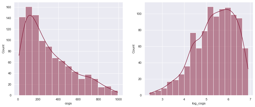
As we can see, the log transformation made the distribution of Cost of Goods Sold (cogs) more normally distributed (or less right-skewed). This will benefit models like linear regression as their weights/coefficients won't be strongly influenced by outliers that caused the initial skewness.
As an aside, since we'll be comparing plots next to each other like this many times during the article, we'll just use this helper function from now on:
def plot_hist(data1, data2):
fig, (ax1, ax2) = plt.subplots(1, 2, figsize=(15,6))
sns.histplot(data1, ax=ax1, kde=True)
sns.histplot(data2, ax=ax2, kde=True);Numeric Scaling
The columns in a dataset are usually on different scales. In our dataset, for example, 'gross income' and 'Rating' are on very different scales (as seen below). To correct for this we can perform 'normalization' to put both columns on a 0-1 scale.
Why do we do this? When predictor variables are on very different scales, models like linear regression may bias coefficients to variables on a larger scale. So we correct for this by normalizing those numeric variables.
We can normalize a variable in many ways, but the most common way to do it is by using the min-max scaler (shown below the plots). The formula is shown below - for each value in the column, we subtract the minimum value of the column and divide the resulting number with the range of the column ($max - min$).
$$\large X_{scaled} = \frac{X - X_{min}}{X_{max} - X_{min}}$$
We can see the range of gross income and Rating currently in our dataset:
gincome = df["gross income"]
rating = df["Rating"]
print(f'Gross income range: {gincome.min()} to {gincome.max()}')
print(f'Rating range: {rating.min()} to {rating.max()}')
plot_hist(gincome, rating)Gross income range: 0.5085 to 49.65
Rating range: 4.0 to 10.0
We can see the difference in scale after applying normalization below.
df[["gross income", "Rating"]] = MinMaxScaler().fit_transform(df[["gross income", "Rating"]])
plot_hist(df['gross income'], df['Rating'])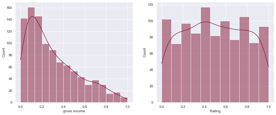
Notice the graphs look the same but the scaling on the x-axis is between 0 and 1 now.
Categorical Variable Handling
One-hot encoding
Machine learning models can only handle numeric variables. Therefore we must encode categorical variables as numeric ones. The easiest way to do this is to 'one-hot-encode' them which means we create $n$ indicator variables for a categorical column with $n$ categories. The below code shows how we can one-hot-encode two categorical columns - Gender and Payment.
pd.get_dummies(df[['Gender','Payment']]).head()| Gender_Female | Gender_Male | Payment_Cash | Payment_Credit card | Payment_Ewallet | |
|---|---|---|---|---|---|
| 0 | 1 | 0 | 0 | 0 | 1 |
| 1 | 1 | 0 | 1 | 0 | 0 |
| 2 | 0 | 1 | 0 | 1 | 0 |
| 3 | 0 | 1 | 0 | 0 | 1 |
| 4 | 0 | 1 | 0 | 0 | 1 |
But there are problems with this approach. If we have a column with 1000 categories, one-hot-encoding that one column will create 1000 new columns! That's a lot! You're feeding the model way too much information and it naturally is much harder to find patterns. When we have too much dimensionality, our model will take much longer to train and find the optimal predictor weights.
Target encoding
To resolve this, we can use target encoding. Target encoding does not create additional columns. The idea is simple - For each unique category, the average value of the target variable (assuming it is either continuous or binary) is calculated and that becomes the value for the respective category in the categorical column.
Let's look at a simple example first before we apply it to our dataset. We have two columns - the target and the predictor variable. Our goal is to encode the predictor variable (a categorical column) into a numeric variable that can be used by the model. To do this we simply group by the predictor variable to get the mean target value for each predictor category. So for predictor a the encoded value will be the mean of 1 and 5, which is 3. For b it is the mean of 4 and 6, which is 5. Now our categorical column is a numeric column!
target = [1, 4, 5, 6]
predictor = ['a', 'b', 'a', 'b']
target_enc_df = pd.DataFrame(data={'target':target, 'predictor':predictor})
means = target_enc_df.groupby('predictor')['target'].mean()
target_enc_df['predictor_encoded'] = target_enc_df['predictor'].map(means)
target_enc_df| target | predictor | predictor_encoded | |
|---|---|---|---|
| 0 | 1 | a | 3 |
| 1 | 4 | b | 5 |
| 2 | 5 | a | 3 |
| 3 | 6 | b | 5 |
Next, we use target encoding in our supermarket dataset. For the example below, we use Product line as the categorical column that is target encoded, and Rating is the target variable, which is a continuous variable.
means = df.groupby('Product line')['Rating'].mean()
df['Product line target encoded'] = df['Product line'].map(means)
df[['Product line','Product line target encoded','Rating']]| Product line | Product line target encoded | Rating | |
|---|---|---|---|
| 0 | Health and beauty | 0.506134 | 0.850000 |
| 1 | Electronic accessories | 0.481313 | 0.933333 |
| 2 | Home and lifestyle | 0.479139 | 0.566667 |
| 3 | Health and beauty | 0.506134 | 0.733333 |
| 4 | Sports and travel | 0.484151 | 0.216667 |
| ... | ... | ... | ... |
| 998 | Home and lifestyle | 0.479139 | 0.016667 |
| 999 | Fashion accessories | 0.514341 | 0.433333 |
| 1000 | Fashion accessories | 0.514341 | 0.433333 |
| 1001 | Electronic accessories | 0.481313 | 0.800000 |
| 1002 | Electronic accessories | 0.481313 | 0.250000 |
1003 rows × 3 columns
Target encoding does have its downsides - when a category only appears once, the mean value of that category is the value itself (the mean of one number is the number itself). In general, it isn’t always a good idea to rely on an average when the number of values used in the average is low. It leads to problems with generalizing results in the training dataset to the testing dataset, or data the model isn't trained on.
The takeaway from this section is to attempt one-hot-encoding if dimensionality won't be a problem. If it is a problem, you can use other approaches like target encoding.
Missing Value Handling
Predictive modeling can be thought of as extracting the right signals from a dataset. Missing values can either be a source of signal themselves (when values are not missing at random) or they can be an absence of signal (when values are missing at random).
Note
Note: the data was modified to contain missing values so we could discuss this topic. If you get a fresh copy from Kaggle, it shouldn't have any missing values.
For example, let's say we have some population data and we add a column called has_license indicating whether a person has a driver's license or not. We will notice missing values - a disproportionate amount of them being people under the age of 18. This is a case where values are NOT missing at random. Now if we have a few missing values in the Gender column caused by data entry issues, those values are likely to be missing at random.
Why is this important? If we have missing data that isn't random, we know why the values are missing, and it can be explained by the dataset, we can simply encode that as an indicator variable indicating. This would allow the model to easily figure it out. However, if the explanation for why they are missing is not explained by the dataset, then we are in murky territory and the handling of such a case requires more advanced attention.
When data is missing at random, we have a loss of information, but we hope we can fill in those gaps based on information from other features.
The least we can do is remove the rows with missing data, as most models don't handle missing data. Since columns with too many missing values don't usually provide a helpful signal, we could remove them based on a threshold condition for missingness (shown below).
But before we fill in missing values, it may be useful to first visualize the missing values using Seaborn.
plt.figure(figsize=(15, 15))
sns.heatmap(df.isnull(), cbar=False);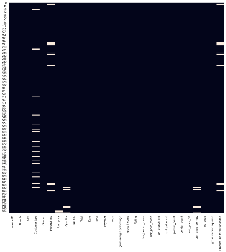
We see there are missing values in a few columns - Customer type, a categorical column, having the most missing values. Usually, columns with too many missing values don't provide enough signal for prediction - so some practitioners decide to remove those columns by setting a threshold for "missingness". In the below code chunk we set the threshold to be 70% and remove columns and rows that meet these conditions.
I do not recommend this strategy - there may still be useful information in these columns/rows and I would let the feature selection process decide whether or not to keep/remove columns. Regardless, if you simply want to build a quick baseline model you may employ this strategy.
Here's how you might remove missing values for a certain threshold:
threshold = 0.7
# Dropping columns with missing value rate higher than threshold
df = df[df.columns[df.isnull().mean() < threshold]]
# Dropping rows with missing value rate higher than threshold
df = df.loc[df.isnull().mean(axis=1) < threshold]Alternatively (preferably), we can impute missing values with a single value such as the mean or median of the column. For categorical columns, we could impute missing values with the mode, or most frequent category in the column.
# Filling missing values with medians of the columns
df = df.fillna(df.median())
# Fill remaining columns - categorical columns - with mode
df = df.apply(lambda x:x.fillna(x.value_counts().index[0]))Now we see no more missing values in the dataset!
plt.figure(figsize=(15, 15))
sns.heatmap(df.isnull(), cbar=False);
There are more complicated imputation techniques beyond the scope of this article, but this should be enough to get you started. If interested in further exploration in handling missing data, I highly recommend checking out Missing Data by Paul D. Allison.
Date-Time Decomposition
Date-time decomposition is quite simply breaking down a date variable into its constituents. We do this as the model needs to works with numeric variables.
# Convert to datetime object
df['Date'] = pd.to_datetime(df['Date'])
df[['Date']].head()| Date | |
|---|---|
| 0 | 2019-01-05 |
| 1 | 2019-03-08 |
| 2 | 2019-03-03 |
| 3 | 2019-01-27 |
| 4 | 2019-02-08 |
# Decomposition
df['Year'] = df['Date'].dt.year
df['Month'] = df['Date'].dt.month
df['Day'] = df['Date'].dt.day
df[['Year','Month','Day']].head()| Year | Month | Day | |
|---|---|---|---|
| 0 | 2019 | 1 | 5 |
| 1 | 2019 | 3 | 8 |
| 2 | 2019 | 3 | 3 |
| 3 | 2019 | 1 | 27 |
| 4 | 2019 | 2 | 8 |
What we've just done is separate out the date column which was in the format "year-month-day" into individual columns, namely year, month, and day. This is information that the model can now use to make predictions, as the new columns are numeric.
Domain-based Approach
There isn't a strict boundary between domain-based and checklist-based approaches to feature engineering. The distinction, I would say, is quite subjective - with domain-based features, you still apply a lot of the techniques we've already discussed, but with a heavy emphasis on domain knowledge.
Domain-based features will involve a lot of ad-hoc metrics like ratios, formulas. etc. We will see examples of this in the case study example below.
Case Study Example - Movie Box Office Data
Now that we have learned several feature engineering techniques, let's apply them!
For our case study, we will be working movie box office data. You can find more information about the dataset by clicking here.
Normally, our first step would be to conduct exploratory data analysis on the dataset, but since this is an article about feature engineering, we will focus on that. Note, a lot of the ideas for feature engineering shown below were inspired by a Kaggle kernel linked here.
df = pd.read_csv('data/movies.csv')
df.head()| id | belongs_to_collection | budget | genres | homepage | imdb_id | original_language | original_title | overview | popularity | ... | release_date | runtime | spoken_languages | status | tagline | title | Keywords | cast | crew | revenue | |
|---|---|---|---|---|---|---|---|---|---|---|---|---|---|---|---|---|---|---|---|---|---|
| 0 | 1 | [{'id': 313576, 'name': 'Hot Tub Time Machine ... | 14000000 | [{'id': 35, 'name': 'Comedy'}] | NaN | tt2637294 | en | Hot Tub Time Machine 2 | When Lou, who has become the "father of the In... | 6.575393 | ... | 2/20/15 | 93.0 | [{'iso_639_1': 'en', 'name': 'English'}] | Released | The Laws of Space and Time are About to be Vio... | Hot Tub Time Machine 2 | [{'id': 4379, 'name': 'time travel'}, {'id': 9... | [{'cast_id': 4, 'character': 'Lou', 'credit_id... | [{'credit_id': '59ac067c92514107af02c8c8', 'de... | 12314651 |
| 1 | 2 | [{'id': 107674, 'name': 'The Princess Diaries ... | 40000000 | [{'id': 35, 'name': 'Comedy'}, {'id': 18, 'nam... | NaN | tt0368933 | en | The Princess Diaries 2: Royal Engagement | Mia Thermopolis is now a college graduate and ... | 8.248895 | ... | 8/6/04 | 113.0 | [{'iso_639_1': 'en', 'name': 'English'}] | Released | It can take a lifetime to find true love; she'... | The Princess Diaries 2: Royal Engagement | [{'id': 2505, 'name': 'coronation'}, {'id': 42... | [{'cast_id': 1, 'character': 'Mia Thermopolis'... | [{'credit_id': '52fe43fe9251416c7502563d', 'de... | 95149435 |
| 2 | 3 | NaN | 3300000 | [{'id': 18, 'name': 'Drama'}] | http://sonyclassics.com/whiplash/ | tt2582802 | en | Whiplash | Under the direction of a ruthless instructor, ... | 64.299990 | ... | 10/10/14 | 105.0 | [{'iso_639_1': 'en', 'name': 'English'}] | Released | The road to greatness can take you to the edge. | Whiplash | [{'id': 1416, 'name': 'jazz'}, {'id': 1523, 'n... | [{'cast_id': 5, 'character': 'Andrew Neimann',... | [{'credit_id': '54d5356ec3a3683ba0000039', 'de... | 13092000 |
| 3 | 4 | NaN | 1200000 | [{'id': 53, 'name': 'Thriller'}, {'id': 18, 'n... | http://kahaanithefilm.com/ | tt1821480 | hi | Kahaani | Vidya Bagchi (Vidya Balan) arrives in Kolkata ... | 3.174936 | ... | 3/9/12 | 122.0 | [{'iso_639_1': 'en', 'name': 'English'}, {'iso... | Released | NaN | Kahaani | [{'id': 10092, 'name': 'mystery'}, {'id': 1054... | [{'cast_id': 1, 'character': 'Vidya Bagchi', '... | [{'credit_id': '52fe48779251416c9108d6eb', 'de... | 16000000 |
| 4 | 5 | NaN | 0 | [{'id': 28, 'name': 'Action'}, {'id': 53, 'nam... | NaN | tt1380152 | ko | 마린보이 | Marine Boy is the story of a former national s... | 1.148070 | ... | 2/5/09 | 118.0 | [{'iso_639_1': 'ko', 'name': '한국어/조선말'}] | Released | NaN | Marine Boy | NaN | [{'cast_id': 3, 'character': 'Chun-soo', 'cred... | [{'credit_id': '52fe464b9251416c75073b43', 'de... | 3923970 |
5 rows × 23 columns
Filling missing values
First, let's handle missing values. We visualize them using Seaborn and then fill in numeric missing values with the median and categorical missing values with the mode.
plt.figure(figsize=(15, 15))
sns.heatmap(df.isnull(), cbar=False);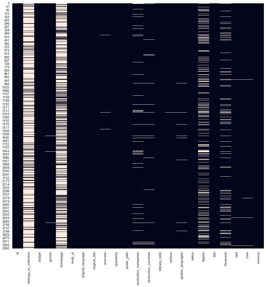
We will fill in the missing numeric variables with the median and the categorical column with the mode. We'll address the categorical missing values after we finish feature engineering other columns (at the very end).
There isn't a hard science to choosing what missing value imputation approach you take. Most practitioners test multiple missing value imputation techniques and decide on the one that gets the best evaluation score.
Decomposing Date
And now we can decompose the date column to its attributes. Note we encode month and day as string variables as there isn't a numeric relationship within them. Days and months have fixed bounds (month doesn't go above 12, the day doesn't go above 31). Day number 10 and 31 are simply different days (think of them as categories).
Let's put year, month, and day into their own columns in the dataframe:
df['release_date'] = pd.to_datetime(df['release_date'])
# decomposition
df['Year'] = df['release_date'].dt.year
df['Month'] = df['release_date'].dt.month.astype(str)
df['Day'] = df['release_date'].dt.day.astype(str)
df[['Year','Month','Day']].head()| Year | Month | Day | |
|---|---|---|---|
| 0 | 2015 | 2 | 20 |
| 1 | 2004 | 8 | 6 |
| 2 | 2014 | 10 | 10 |
| 3 | 2012 | 3 | 9 |
| 4 | 2009 | 2 | 5 |
Adjusting budget
Since the budget is highly right-skewed, we take the logarithm of the budget to adjust for it. Note we take the logarithm of the budget + 1 as a lot of movies have a budget of $0 and we cannot take the logarithm of 0.
df['log_budget'] = np.log(df['budget'] + 1)
plot_hist(df['budget'], df['log_budget'])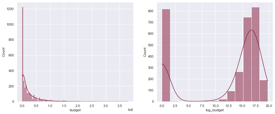
Encoding inflation
We know the budget increases yearly to some extent due to inflation. We can encode that using a simple inflation formula as follows:
$$\large InflationBudget_i = Budget_i \big( 1 + \frac{1.8}{100} \times (MaxYear - Year_i) \big) $$
Where $i$ is each row and $MaxYear$ is the maximum year of the dataset (2018 in our case). Here's creating it for our dataframe:
df['inflation_budget'] = df['budget'] * (1 + (1.8 / 100) * (2018 - df['Year']))
plot_hist(df['budget'], df['inflation_budget'])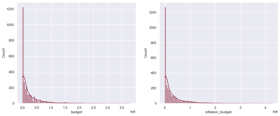
Other interesting features
Based on domain knowledge, we can create some useful ratio variables as shown below.
df['budget_runtime_ratio'] = df['budget'] / df['runtime']
df['budget_popularity_ratio'] = df['budget'] / df['popularity']
df['budget_year_ratio'] = df['budget'] / (df['Year'] * df['Year'])
df['releaseYear_popularity_ratio'] = df['Year'] / df['popularity']Indicator variables
We encode an indicator variable indicating whether a movie has a homepage or not, and whether the movie was in English:
# Has a homepage
df['has_homepage'] = 1
df.loc[pd.isnull(df['homepage']), "has_homepage"] = 0
# Was in English
df['is_english'] = np.where(df['original_language']=='en', 1, 0)And now we can fill in the missing categorical column values.
# Fill remaining columns - categorical columns - with mode
df = df.apply(lambda x: x.fillna(x.value_counts().index[0]))We subset the data frame to include only the variables we want.
engineered_df = df[['budget_runtime_ratio',
'budget_popularity_ratio',
'budget_year_ratio',
'releaseYear_popularity_ratio',
'inflationBudget',
'Year',
'Month',
'is_english',
'has_homepage',
'budget',
'popularity',
'runtime',
'revenue']]We one-hot-encode the categorical columns. In our case, we only have one categorical column - month.
engineered_df = engineered_df.replace([np.inf, -np.inf], np.nan).dropna(axis=1)
engineered_df = pd.get_dummies(engineered_df)Our new data frame looks like this
engineered_df.head()| budget_popularity_ratio | budget_year_ratio | releaseYear_popularity_ratio | inflationBudget | Year | is_english | has_homepage | budget | popularity | runtime | ... | Month_11 | Month_12 | Month_2 | Month_3 | Month_4 | Month_5 | Month_6 | Month_7 | Month_8 | Month_9 | |
|---|---|---|---|---|---|---|---|---|---|---|---|---|---|---|---|---|---|---|---|---|---|
| 0 | 2.129150e+06 | 3.448085 | 306.445562 | 14756000.0 | 2015 | 1 | 0 | 14000000 | 6.575393 | 93.0 | ... | 0 | 0 | 1 | 0 | 0 | 0 | 0 | 0 | 0 | 0 |
| 1 | 4.849134e+06 | 9.960120 | 242.941630 | 50080000.0 | 2004 | 1 | 0 | 40000000 | 8.248895 | 113.0 | ... | 0 | 0 | 0 | 0 | 0 | 0 | 0 | 0 | 1 | 0 |
| 2 | 5.132194e+04 | 0.813570 | 31.321933 | 3537600.0 | 2014 | 1 | 1 | 3300000 | 64.299990 | 105.0 | ... | 0 | 0 | 0 | 0 | 0 | 0 | 0 | 0 | 0 | 0 |
| 3 | 3.779604e+05 | 0.296432 | 633.713561 | 1329600.0 | 2012 | 0 | 1 | 1200000 | 3.174936 | 122.0 | ... | 0 | 0 | 0 | 1 | 0 | 0 | 0 | 0 | 0 | 0 |
| 4 | 0.000000e+00 | 0.000000 | 1749.893299 | 0.0 | 2009 | 0 | 0 | 0 | 1.148070 | 118.0 | ... | 0 | 0 | 1 | 0 | 0 | 0 | 0 | 0 | 0 | 0 |
5 rows × 23 columns
Now that our dataset is ready, we can go through the process of selecting useful features (feature selection) and make predictions.
Prediction
To prove feature engineering works, and improves the performance of the model, we can build a simple regression model to predict the revenue of movies.
Normally we pick what features to use via a process called feature selection, however, since this article is focused on feature engineering, we will employ a simple process of selecting features: correlation analysis.
By plotting the correlation matrix (below), we see most of the features we created aren't that predictive of revenue. This is what happens most of the time - you build a ton of features, but only a few end up being useful - but those features that are useful make a difference.
From the plot below we will use has_homepage, budget_year_ratio, and is_english in our model, in addition to features that came before feature engineering - budget,runtime and popularity.
plt.figure(figsize=(10, 8))
sns.heatmap(engineered_df.corr());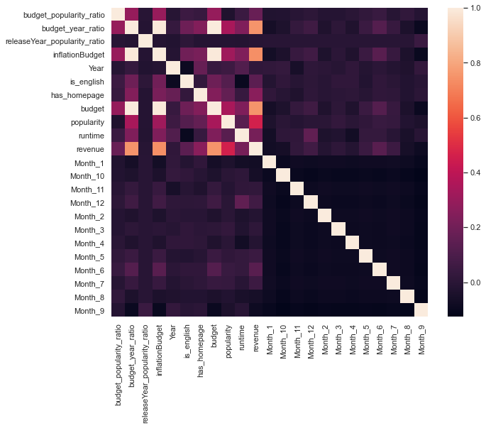
We will use approximately 80% of the dataset for training the baseline and feature engineered models, and compare their performances on the hidden test set.
train_engineered = engineered_df[['budget','runtime','popularity',
'has_homepage','budget_year_ratio','is_english']].iloc[:2500]
train_baseline = engineered_df[['budget','runtime','popularity']].iloc[:2500]
test_engineered = engineered_df[['budget','runtime','popularity',
'has_homepage','budget_year_ratio','is_english']].iloc[2500:]
test_baseline = engineered_df[['budget','runtime','popularity']].iloc[2500:]
target_train = engineered_df['revenue'].iloc[:2500]
target_test = engineered_df['revenue'].iloc[2500:]reg_baseline = LinearRegression().fit(train_baseline, target_train)
reg_predict_baseline = reg_baseline.predict(test_baseline)
reg_engineered = LinearRegression().fit(train_engineered, target_train)
reg_predict_engineered = reg_engineered.predict(test_engineered)
rmse_baseline = np.sqrt(mean_squared_error(target_test, reg_predict_baseline))
rmse_engineered = np.sqrt(mean_squared_error(target_test, reg_predict_engineered))
rmse_difference = rmse_baseline - rmse_engineered
print ("The difference in RMSE is", round(rmse_difference, 2), "dollars")The difference in RMSE is 909146.83 dollarsThe difference is quite stark! The baseline model's — that uses only budget, runtime and popularity as features — predictions are on average $909,146.83 worse than the model where we used our constructed features. We came to that conclusion by comparing the Root Mean Squared Error (RMSE) of both models on the test set.
By using feature engineering, we allowed our model to get a better understanding of our dataset, and therefore make better predictions.
Conclusion
Feature Engineering Pitfalls
Some of the common pitfalls of feature engineering are:
- Overfitting: When we construct too many features, we risk overfitting the data. This is often referred to as the curse of dimensionality. Briefly, the more features a model has the more flexibility it has to establish relationships between the predictor and the target variable. This may sound like a good thing, but if a model has too much flexibility, it will, in a sense, over-optimize on the data it is trained on. This will result in a high-performance score but will perform poorly on hidden data or new data, as new data will have differences not observed in the training data. We have to be mindful of this and take into consideration out of sample testing when evaluating features (during the feature selection step).
- Information leakage: If feature engineering is not done properly it could lead to information leakage. This usually involves the construction of new features using the target variable. Feature engineering must always be done independently of the target variable and must only include predictor variables of interest.
The feature engineering mindset
The feature engineering mindset is very experimental. Generally, quantity is valued over quality. Quality comes into play when we deal with feature selection which happens after feature engineering. We may have some direction as to what features may be useful, but we should not let our bias come into play - construct as many relevant features as possible from your data (computation and time permitting of course) and follow it up with a robust feature selection process to weed out bad features.
Further learning:
Many data science and machine learning courses contain sections on feature engineering. Here's a great course to check out:
Meet the Authors

Bassim is a Data Scientist at NoviSci where he helps solve hard epidemiology problems using numerous statistical tools.

Founder of LearnDataSci