Sentiment Analysis on Reddit News Headlines with Python’s Natural Language Toolkit (NLTK)
Let's use the Reddit API to grab news headlines and perform Sentiment Analysis
LearnDataSci is reader-supported. When you purchase through links on our site, earned commissions help support our team of writers, researchers, and designers at no extra cost to you.
You should already know:
- Python fundamentals
- Basic machine learning concepts
Learn both interactively through dataquest.io
In the last post, K-Means Clustering with Python, we just grabbed some precompiled data, but for this post, I wanted to get deeper into actually getting some live data.
Using the Reddit API we can get thousands of headlines from various news subreddits and start to have some fun with Sentiment Analysis.
We are going to use NLTK's vader analyzer, which computationally identifies and categorizes text into three sentiments: positive, negative, or neutral.
Article Resources
- Notebook: GitHub
- Libraries: pandas, numpy, nltk, matplotlib, seaborn
Getting Started
First, some imports:
These imports will be cleared up once they are used. The three that are worth mentioning now are pprint, which lets us "pretty-print" JSON and lists, seaborn, which will add styles to the matplotlib graphs, and iPython's display module, which will let us control the clearing of printed output inside loops. More on these below.
NLTK
Before we get started with gathering the data, you will need to install the Natural Language Toolkit (NLTK) python package. To see how to install NLTK, you can go here: http://www.nltk.org/install.html. You'll need to open Python command line and run nltk.download() to grab NLTK's databases.
Reddit API via PRAW
For this tutorial, we'll be using a Reddit API wrapper, called `praw`, to loop through the /r/politics subreddit headlines.
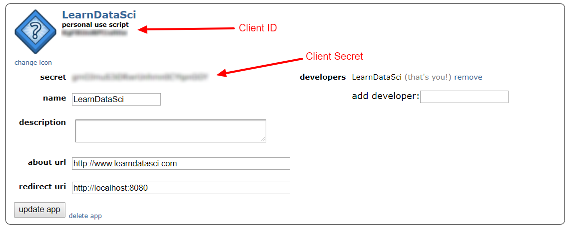
To get started with `praw`, you will need to create a Reddit app and obtain your Client ID and Client Secret.
Making a Reddit app
Simply follow these steps:
- Log into your account
- Navigate to https://www.reddit.com/prefs/apps/
- Click on the button that says "are you a developer? create an app..."
- Enter a name (username works)
- Select "script"
- Use http://localhost:8080 as a redirect URI
- Once you click "create app", you'll see where your Client ID and Client Secret are.
Now to get started with praw, we need to first create a Reddit client.
Just replace your details in the following lines (without carets < >):
Let's define a set for our headlines so we don't get duplicates when running multiple times:
Now, we can iterate through the /r/politics subreddit using the API client:
We're iterating over the "new" posts in /r/politics, and by setting the limit to None we can get up to 1000 headlines. This time we only received 965 headlines.
PRAW does a lot of work for us. It lets us use a really simple interface while it handles a lot of tasks in the background, like rate limiting and organizing the JSON responses.
Unfortunately, without some more advanced tricks we can't go past 1000 results since Reddit cuts off at that point. We can run this loop multiple times and keep adding new headlines to our set, or we can implement a streaming version. There's also a way to take advantage of Reddit's search with time parameters, but let's move on to the Sentiment Analysis of our headlines for now.
Labeling our Data
NLTK’s built-in Vader Sentiment Analyzer will simply rank a piece of text as positive, negative or neutral using a lexicon of positive and negative words.
We can utilize this tool by first creating a Sentiment Intensity Analyzer (SIA) to categorize our headlines, then we'll use the polarity_scores method to get the sentiment.
We'll append each sentiment dictionary to a results list, which we'll transform into a dataframe:
| compound | headline | neg | neu | pos | |
|---|---|---|---|---|---|
| 0 | -0.5267 | DOJ watchdog reportedly sends criminal referra... | 0.254 | 0.746 | 0.000 |
| 1 | 0.0000 | House Dems add five candidates to ‘Red to Blue... | 0.000 | 1.000 | 0.000 |
| 2 | 0.0000 | DeveloperTown co-founder launches independent ... | 0.000 | 1.000 | 0.000 |
| 3 | 0.5267 | Japanese PM Praises Trump for North Korea Brea... | 0.000 | 0.673 | 0.327 |
| 4 | 0.0000 | Democrats Back 'Impeach Trump' Candidates, Pol... | 0.000 | 1.000 | 0.000 |
Our dataframe consists of four columns from the sentiment scoring: Neu, Neg, Pos and compound. The first three represent the sentiment score percentage of each category in our headline, and the compound single number that scores the sentiment. `compound` ranges from -1 (Extremely Negative) to 1 (Extremely Positive).
We will consider posts with a compound value greater than 0.2 as positive and less than -0.2 as negative. There's some testing and experimentation that goes with choosing these ranges, and there is a trade-off to be made here. If you choose a higher value, you might get more compact results (less false positives and false negatives), but the size of the results will decrease significantly.
Let's create a positive label of 1 if the compound is greater than 0.2, and a label of -1 if compound is less than -0.2. Everything else will be 0.
| compound | headline | neg | neu | pos | label | |
|---|---|---|---|---|---|---|
| 0 | -0.5267 | DOJ watchdog reportedly sends criminal referra... | 0.254 | 0.746 | 0.000 | -1 |
| 1 | 0.0000 | House Dems add five candidates to ‘Red to Blue... | 0.000 | 1.000 | 0.000 | 0 |
| 2 | 0.0000 | DeveloperTown co-founder launches independent ... | 0.000 | 1.000 | 0.000 | 0 |
| 3 | 0.5267 | Japanese PM Praises Trump for North Korea Brea... | 0.000 | 0.673 | 0.327 | 1 |
| 4 | 0.0000 | Democrats Back 'Impeach Trump' Candidates, Pol... | 0.000 | 1.000 | 0.000 | 0 |
We have all the data we need to save, so let's do that:
We can now keep appending to this csv, but just make sure that if you reassign the headlines set, you could get duplicates. Maybe add a more advanced saving function that reads and removes duplicates before saving.
Dataset Info and Statistics
Let's first take a peak at a few positive and negative headlines:
Now let's check how many total positives and negatives we have in this dataset:
The first line gives us raw value counts of the labels, whereas the second line provides percentages with the normalize keyword.
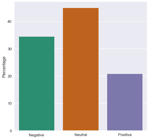
For fun, let's plot a bar chart:
The large number of neutral headlines is due to two main reasons:
- The assumption that we made earlier where headlines with compound value between 0.2 and -0.2 are considered neutral. The higher the margin, the larger the number of neutral headlines.
- We used general lexicon to categorize political news. The more correct way is to use a political-specific lexicon, but for that we would either need a human to manually label data, or we would need to find a custom lexicon already made.
Another interesting observation is the number of negative headlines, which could be attributed to the media’s behavior, such as the exaggeration of titles for clickbait. Another possibility is that our analyzer produced a lot of false negatives.
There's definitely places to explore for improvements, but let's move on for now.
Tokenizers and Stopwords
Now that we gathered and labeled the data, let's talk about some of the basics of preprocessing data to help us get a clearer understanding of our dataset.
First of all, let’s talk about tokenizers. Tokenization is the process of breaking a stream of text up into meaningful elements called tokens. You can tokenize a paragraph into sentences, a sentence into words and so on.
In our case, we have headlines, which can be considered sentences, so we will use a word tokenizer:
As you can see, the previous tokenizer, treats punctuation as words, but you might want to get rid of the punctuation to further normalize the data and reduce feature size. If that’s the case, you will need to either remove the punctuation, or use another tokenizer that only looks at words, such as this one:
There's quite a few tokenizers, and you can view them all here: http://www.nltk.org/api/nltk.tokenize.html. There's probably one that fits the bill more than others. The TweetTokenizer is a good example.
In the above tokens you'll also notice that we have a lot of words like ’the, ’is’, ’and’, ’what’, etc. that are somewhat irrelevant to text sentiment and don't provide any valuable information. These are called stopwords.
We can grab a simple list of stopwords from NLTK:
This is a simple English stopword list that contains most of the common filler words that just add to our data size for no additional info. Further down the line, you'll most likely use a more advanced stopword list that's ideal for your use case, but NLTK's is a good start.
Word Distributions
Let's start by creating a function that will read a list of headlines and perform lowercasing, tokenizing, and stopword removal:
Positive Words
We can grab all of the positive label headlines from our dataframe, hand them over to our function, then call NLTK's `FreqDist` function to get the most common words in the positive headlines:
Now, let’s see the frequency of some of the tops words in the positive set:
Interestingly the most positive headline word is 'trump'!
Seeing that some of the other top positive words are having to do with with the Russia investigation, it's most likely the case that "trump" + "investigation news" is mostly seen as positive, but as we'll see in the negative word section, a lot of the same words appear so it's not definitive.
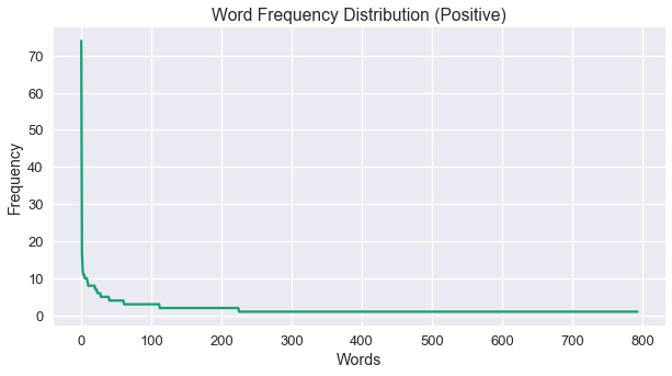
Let’s look at more macroscopic side by plotting the frequency distribution and try to examine the pattern of words and not each word specifically.
The above chart is showing the frequency patterns, where the y-axis is the frequency of the words and in x-axis is the words ranked by their frequency. So, the most frequent word, which in our case is ‘trump’, is plotted at $(1, 74)$.
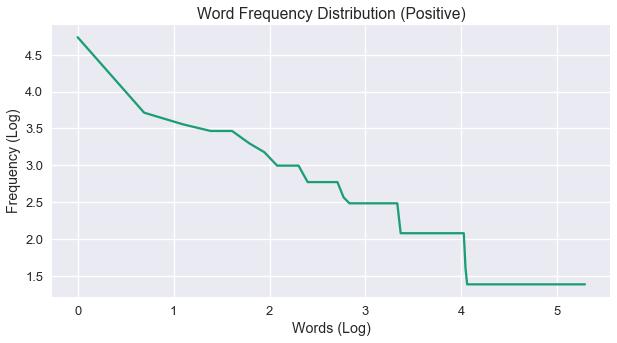
For some of you, that plot may seem a bit familiar. That’s because it’s seems to be following the power-law distribution. So, to visually confirm it, we can use a log-log plot:
As expected, an almost straight line with a heavy tail (noisy tail). This shows that our data fits under the Zipf’s Law. In other words, the above plot shows that in our word distribution a vast minority of the words appear the most, while the majority of words appear less.
Negative Words
Now that we have examined the positive words, it’s time to shift towards the negative ones. Let's get and process the negative text data:
Well, the President does it again. He's also the top negative word. An interesting addition to the list are the words ‘syria’ and 'war'.
This post is being updated right when the first big strike on Syria occurred, so it seems pretty obvious why that would be seen as negative.
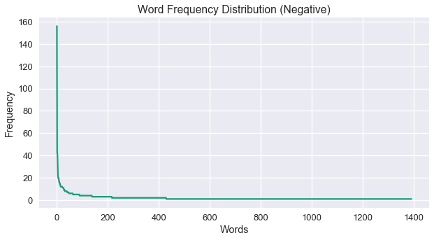
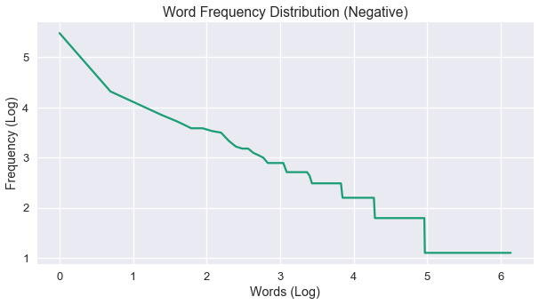
Interestingly, as noted above, we see some of the same words, like 'comey' and 'mueller', that appeared in the positive set. Some more analysis is needed to pin down the differences to see if we can separate more accurately, but for now let's move on to some of the plots for negative word distributions:
Negative distribution fits under the Zipf Law as well. A bit of more smooth slope, but the heavy tail is definitely there. The conclusion to be drawn here, is the exact same as the previous one shown in positive distribution.
Conclusion
As you can see, the Reddit API makes it extremely easy to compile a lot of news data fairly quickly. It's definitely worth the time and effort to enhance the data collection steps since it's so simple to get thousands of rows of political headlines to use for further analysis and prediction.
There's still a lot that could be engineered in regards to data mining, and there's still a lot to do with the data retrieved. The the next tutorial we will continue our analysis by the dataset to construct and train a sentiment classifier.


