

Data Scientist, Ph. D. Student in Computational Neuroscience
Sigmoid Function
What is the sigmoid function?
A sigmoid function is a mathematical function with a characteristic "S"-shaped curve or sigmoid curve. It transforms any value in the domain $(-\infty, \infty)$ to a number between 0 and 1.
Applications
The sigmoid function's ability to transform any real number to one between 0 and 1 is advantageous in data science and many other fields such as:
- In deep learning as a non-linear activation function within neurons in artificial neural networks to allows the network to learn non-linear relationships between the data
- In binary classification, also called logistic regression, the sigmoid function is used to predict the probability of a binary variable.
Issues with the sigmoid function
Although the sigmoid function is prevalent in the context of gradient descent, the gradient of the sigmoid function is in some cases problematic. The gradient vanishes to zero for very low and very high input values, making it hard for some models to improve.
For example, during backpropagation in deep learning, the gradient of a sigmoid activation function is used to update the weights & biases of a neural network. If these gradients are tiny, the updates to the weights & biases are tiny and the network will not learn.
Alternatively, other non-linear functions such as the Rectified Linear Unit (ReLu) are used, which do not show these flaws.
Other learning resources
Week three of the Supervised Machine Learning course on Coursera discusses the sigmoid function in detail, including an example using logistic regression.
Mathematical definition
We typically denote the sigmoid function by the greek letter $\sigma$ (sigma) and define as
$$\Large \sigma(x) = \frac{1}{1+e^{-x}}$$
Where
- $x$ is the input to the sigmoid function
- $e$ is [Euler's number](https://en.wikipedia.org/wiki/E_(mathematical_constant) ($e = 2.781...$)
We'll explore the output of the sigmoid function in a programming example towards the end of the article.
Limits of the sigmoid function
If the input $x$ to the sigmoid function is a small negative number, the output is very close to 0. For example:
$$\begin{align} \Large \sigma(-4) &= \frac{1}{1+e^{-(-4)}} \\[1em] &= 0.01798621 \end{align}$$
Indeed, we can use the limit to show that $\sigma(x)$ approaches 0 as $x$ tends to $-\infty$:
$$\begin{align} \Large \lim_{x\to-\infty} \sigma(x) &= \lim_{x\to-\infty} \frac{1}{1+e^{-x}} \\[1em] &= \lim_{x\to-\infty} \frac{1}{1+e^{\infty}} \\[1em] &= 0 \end{align}$$
If $x$ is a large positive number, then the output is very close to 1:
$$ \begin{align} \Large \sigma(4) &= \frac{1}{1+e^{-(4)}} \\[1em] &= 0.9820138 \end{align} $$
Again, we can use the limit to show that $\sigma(x)$ approaches 1 as $x$ tends to $\infty$:
$$\begin{align} \Large \lim_{x\to\infty} \sigma(x) &= \lim_{x\to\infty} \frac{1}{1+e^{-x}} \\[1em] &= \lim_{x\to\infty} \frac{1}{1+e^{-\infty}} \\[1em] &= 1 \end{align} $$
If $x$ is exactly 0, the output is $0.5$:
$$\begin{align} \Large \sigma(0) &= \frac{1}{1+e^{-(0)}} \\[1em] &= 0.5 \end{align}$$
Now that we've seen how the sigmoid function behaves at its limits let's move on to its derivative.
Derivative of the sigmoid function
Whether it's about training a neural network with a sigmoid activation function or fitting a logistic regression model to data, calculating the derivative of the sigmoid function is very important, as it tells us how to optimize the parameters of our model with gradient descent to improve performance.
The derivative of the sigmoid function is:
$$\Large \frac{d}{dx}\sigma(x) = \sigma(x)(1-\sigma(x))$$
This expression of the derivative is very convenient since, in most use cases, we have already calculated $s(x)$ in our model before attempting gradient descent (e.g. during the feedforward step in neural networks). If we want to apply gradient descent now, we can insert $s(x)$ into two spots of the derivative equation without any high calculation costs.
To arrive at this derivative, we must first recall the chain rule.
Chain Rule
The derivative of a compositional function — a function within another function — e.g. $h(x) = f(g(x))$, is given by first taking the derivative of the outer function $f$ multiplied by the derivative of the inner function $g$.
Suppose we have the compositional function
$$h(x) = f(g(x))$$
Then according to the chain rule, we have:
$$h'(x) = f'(g(x)) \cdot g'(x)$$
The above formula can be rewritten as a generalized derivative formula as follows:
Let $u = g(x)$, then $$\frac{d}{dx}[f(u)] = f'(u)\frac{du}{dx}$$
We'll use this version to show the chain rule step in the next equation.
Taking the derivative of the sigmoid function
The following equation walks you through each step needed to take the derivative of the sigmoid function. Take note of steps 3-6, which utilize the chain rule, and steps 9-11, which use the algebraic trick of adding and subtracting one from the numerator to get the desired form for cancelation of terms.
$$\begin{align} \Large \frac{d}{dx}\sigma(x) &= \frac{d}{dx} \left[ \frac{1}{1+e^{-x}}\right] \\[1em] &= \frac{d}{dx} \left[ (1+e^{-x} )^{-1} \right] \\[1em] &= \frac{d}{dx} \left[ u^{-1} \right], \quad u = 1+e^{-x} &&\text{Using the chain rule} \\[1em] &= \frac{d}{dx} -u^{-2} \frac{du}{dx} \\[1em] &= -(1+e^{-x})^{-2} \cdot \frac{d}{dx}\left[ 1+e^{-x} \right] \\[1em] &= -( 1+e^{-x} )^{-2} \cdot -e^{-x} \\[1em] &= \frac{-e^-x}{( 1+e^{-x} )^{2}} \\[1em] &= \frac{1}{( 1+e^-x )} \cdot \frac{-e^-x}{1+e^{-x}} \\[1em] &= \frac{1}{( 1+e^-x )} \cdot \frac{(1+e^{-x}) - 1}{1+e^{-x}} &&\text{Add and subtract 1 in the numerator} \\[1em] &= \frac{1}{( 1+e^-x )} \cdot \left( \frac{1+e^{-x}}{1+e^{-x}} - \frac{1}{1+e^{-x}} \right) \\[1em] &= \frac{1}{( 1+e^-x )} \cdot \left( 1 - \frac{1}{1+e^{-x}} \right) \\[1em] &= \sigma(x) \cdot ( 1 - \sigma(x) ) \\[1em] \end{align}$$
Python example
We'll now explore the sigmoid function and its derivative using Python.
First, we'll write two functions that capture, mathematically, the sigmoid function and its derivative:
def sigmoid(x):
return 1 / (1 + np.exp(-x))
def d_sigmoid(x):
return sigmoid(x) * (1 - sigmoid(x))We can now use numpy to create 100 data points to which we can apply the sigmoid and derivative functions:
import numpy as np
# create data
x = np.linspace(-10, 10, 100)
# get sigmoid output
y = sigmoid(x)
# get derivative of sigmoid
d = d_sigmoid(x)Using pandas, we'll create a dataframe for the data to make it easily viewable in a table:
import pandas as pd
df = pd.DataFrame({"x": x, "sigmoid(x)": y, "d_sigmoid(x)": d})
df| x | sigmoid(x) | d_sigmoid(x) | |
|---|---|---|---|
| 0 | -10.000000 | 0.000045 | 0.000045 |
| 1 | -9.797980 | 0.000056 | 0.000056 |
| 2 | -9.595960 | 0.000068 | 0.000068 |
| 3 | -9.393939 | 0.000083 | 0.000083 |
| 4 | -9.191919 | 0.000102 | 0.000102 |
| ... | ... | ... | ... |
| 95 | 9.191919 | 0.999898 | 0.000102 |
| 96 | 9.393939 | 0.999917 | 0.000083 |
| 97 | 9.595960 | 0.999932 | 0.000068 |
| 98 | 9.797980 | 0.999944 | 0.000056 |
| 99 | 10.000000 | 0.999955 | 0.000045 |
100 rows × 3 columns
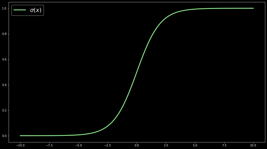
Now, with matplotlib, let's visualize this data. By plotting the sigmoid function, we get the familiar S-curve:
import matplotlib.pyplot as plt
plt.style.use("dark_background")
fig = plt.figure(figsize=(16, 9))
plt.plot(x, y, c="lightgreen", linewidth=3.0, label="$\sigma(x)$")
plt.plot(x, d, c="lightblue", linewidth=3.0, label="$\\frac{d}{dx} \sigma(x)$")
plt.legend(prop={'size': 20})
plt.show()
We'll explore a binary classification problem to see how the sigmoid function is used in context.
Binary classification
Binary classification, also called logistic regression, categorizes new observations into one of two classes. For this example, we'll use simulated data, but for a more in-depth treatment, check out our binary classification term for an example with actual data.
For this example, we'll use the LogisticRegression class from scikit-learn:
from sklearn.linear_model import LogisticRegressionOur example problem will simulate a class of students and test outcomes to determine whether hours spent learning can predict a pass or fail.
We'll create a variable, called hours_spent_learning, to predict the outcome of a binary variable, pass_test ("passed" = 1, "failed" = 0).
# create variable used for prediction
hours_spent_learning = np.linspace(1, 100, 100)
# probability of passing
weights = hours_spent_learning / len(hours_spent_learning)
# create variable we want to predict from hours_spent_learning
pass_test = np.random.binomial(1, weights)To see what's going on with these variables, let's print out the first five values from each:
print('First five values')
print('\thours_spent_learning:\t', hours_spent_learning[:5])
print('\tweights:\t\t', weights[:5])
print('\tpass_test:\t\t', pass_test[:5])First five values
hours_spent_learning: [1. 2. 3. 4. 5.]
weights: [0.01 0.02 0.03 0.04 0.05]
pass_test: [0 0 0 0 0]With an idea of what the data looks like, let's fit the model.
We need to define variables x for the predictor and y for the outcome, after which we can fit a logistic regression model:
x = hours_spent_learning.reshape(-1, 1)
y = pass_test
# fit the model
model = LogisticRegression()
model.fit(x, y)LogisticRegression()And finally we can plot the estimated sigmoid function to predict the binary outcome. As we can see the probability of passing the test increases as more hours are spent learning (see the blue line).
# use the model coefficients to draw the plot
pred = sigmoid(x * model.coef_[0] + model.intercept_[0])
fig = plt.figure(figsize=(16, 9))
plt.plot(x, pred, c="lightblue", linewidth=3.0)
plt.scatter(
x[(y == 1).ravel()],
y[(y == 1).ravel()],
marker=".",
c="lightgreen",
linewidth=1.0,
label="passed",
)
plt.scatter(
x[(y == 0).ravel()],
y[(y == 0).ravel()],
marker=".",
c="red",
linewidth=1.0,
label="failed",
)
plt.axhline(y=0.5, color="orange", linestyle="--", label="boundary")
plt.xlabel("Hours spent learning")
plt.ylabel('p("passing the test")')
plt.legend(frameon=False, loc="best", bbox_to_anchor=(0.5, 0.0, 0.5, 0.5), prop={'size': 20})
plt.show()
Using the decision boundary denoted by the orange line, we can also use the fitted model to predict if a person will pass or fail the test based on the hours spent learning. The convention here is to classify "pass" if the predicted probability is higher than 0.5 or "fail" if lower.
For example:
model.predict([[30]]) # 30 hours spent learning will lead to a fail predictionarray([0])model.predict([[60]]) # 60 hours spent learning will lead to a pass predictionarray([1])Meet the Authors

As a freelancer I am fascinated with all things related to Data Science. My research in academia is based on comparing deep reinforcement learning agents with biological agents.

Founder of LearnDataSci